8.1. OpenModelica inner workings

This chapter gives some ideas on “how OpenModelica works”, that is how does it generate simulation results from a Modelica model. This description of OpenModelica inner workings should also probably extend to other Modelica simulators like Dymola.

Learning objectives

At the end of this chapter, you’ll be able to:

1. Describe the succesive steps involved in a Modelica simulation

2. View the simplified equations with the Transformational Debugger

8.1.1. OpenModelica simulation process

A high level view on how OpenModelica generates the simulation results.

Fig. 8.1 presents the different steps which stand between:

• starting point: the idea of a simulation someone wants to make, hidden in his/her brain.

• objective of the user: simulation results written in a file

Objective: reconstruct the sequence. The different states of transformation of the model should go inside ellipses, while the transforming operations should go inside rectangles.

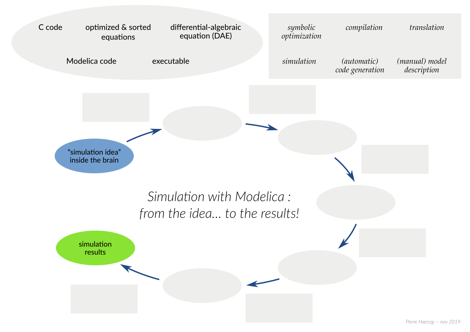
Fig. 8.1 the different steps of a Modelica simulation, to be ordered

Looking at the generated C code

Where are the generated code and compile model (exectuble) located?

Read the blue lines in the “Output” tab of the “Simulation output” window that pops up during simulation. These contain the full path to the model being executed.

• On Linux: /tmp/OpenModelica_username/OMEdit/ModelName/ (with username and ModelName to be adapted)

• On Windows: ?

Also, in recent OpenModelica version, it is necessary to unset the option “Delete intermediate compilation files” which is checked by default. It can be found in the Simulation panel of the general option dialog of OMEdit (menu Tools/Options). Otherwise, all C files are erased once compiled.

Many C files are generated. The C code implementing the ODE equations (after the symbolic manipulation discussed below) can be found in ModelName.c. Relevant lines can be found thanks to the extensive autogenerated comments.

8.1.2. DAE vs ODE

Question

What is the difference between a ODE and a DAE?

8.1.3. Symbolic equation manipulation

Since Modelica is an acausal language, models are formulated as DAEs. However, integrating and ODE is much simpler because it is easy to find explicit integration methods, that is corresponding to a causal equations. In many cases, a symbolic manipulation of the set of equations can enable reformulating a DAE into a ODE.

In OMEdit, it is possible to see the result of these symbolic manipulations thanks to the Transformational Debugger. It can be launched from the toolbar (Fig. 8.2)

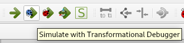
Fig. 8.2 “Simulate with Transformational Debugger” button in OMEdit toolbar

For the Transformational Debugger to display complete information, a dedicated option needs to be activated to keep the trace of all operation transformations. This “Generate Operations” can be found in the Debugger panel of the general option dialog of OMEdit (menu Tools/Options).

Simple ODE example

To get familiar with the tool, it can be applied first to the following simple ODE, which was however formulated in an “acausal way”:

model ODE2_debug "Test how an acausal ODE formulation is solved by OpenModelica. Simulate *with Transformational Debugger*"
  Real x "Position";
  Real v "Velocity";

initial equation
  x = 10.;
  v = 0;

equation
  v = der(x) "definition of velocity";
  der(v) + der(x) + x = 0 "Newton's second law of motion"; 

end ODE2_debug;

Once it is run with the “Simulate with Transformational Debugger” action, the Transformational Debugger pops up as in Fig. 8.3.

The key concept of the output of the equation simplification is the notion of assignment, written with :=. It means that the left hand side can be computed with the right hand side.

Also, assignments are sorted, meaning that they should be executed in this order (ex : first a := 1 and then b := a/2), although in this simple example the main assignments (number 5 and 6) could be flipped. In the next example, this will be visible.

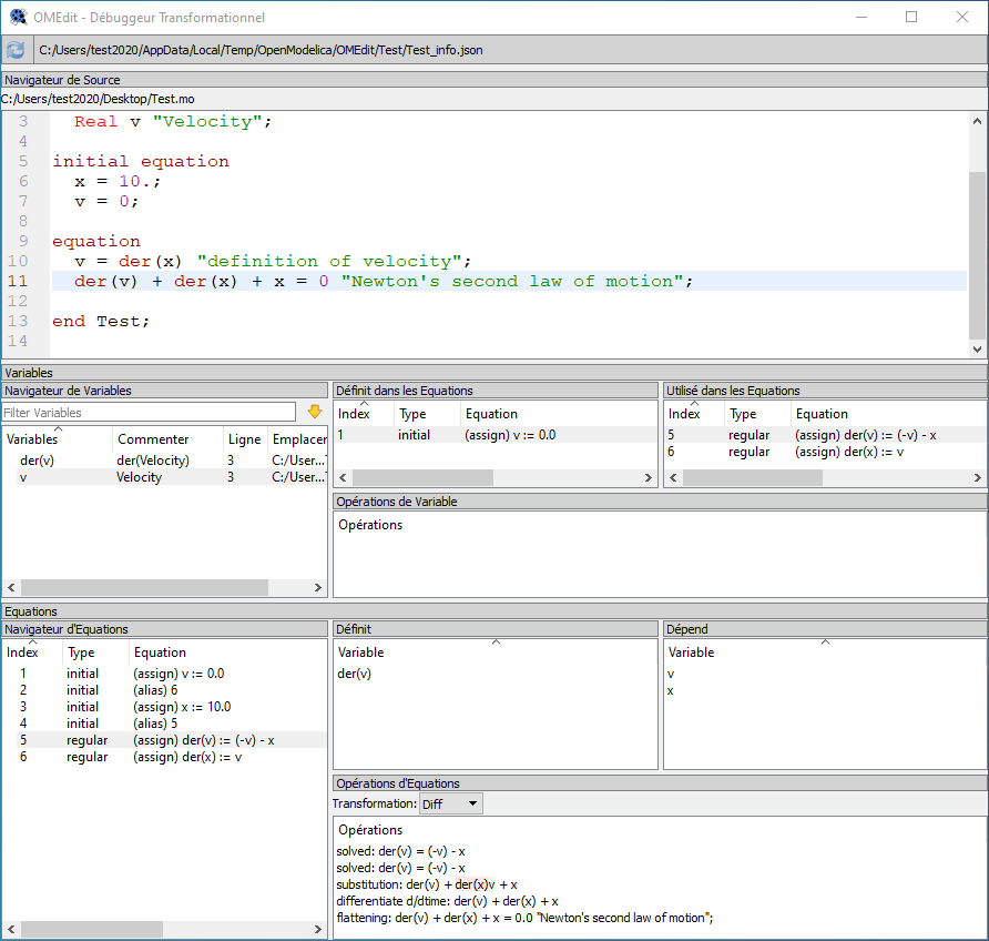
Fig. 8.3 Transformational Debugger showing the sorted and simplified equations of the ODE2_debug model

Electrical circuit example

Then, the Transformational Debugger can be used on a slightly more complex example, such as the electric circuit of Fig. 5.1 in the Physical components in Modelica chapter.

Question

First, try to list on a paper all independant variables (i.e. excluding aliases like capacitor1.v and resistor1.v since they are in parallel) and the equations (differential and algebraic) that govern them. You should find about 5. Think also about the sorting of the equations.

Then, simulate the circuit with the Transformational Debugger and compare you results. OMEdit will find some extra likes the actual resistance of the resistor (because it can be temperature dependant) and the dissipated power. However, the core electrical equations should be equivalent!