4. Describing discrete behaviors

In this session, you’ll learn how to describe in Modelica differential equations which include discrete behaviors (discontinuous changes in the dynamics). Properly describing those in Modelica requires some knowledge of how discontinuities are handled by ODE solvers. In particular, the notion of simulation events.

Main ressource needed:

• Michael Tiller’s online book “Modelica by Example” [Tiller-2014]

  • second chapter Discrete Behavior of the first part “Describing Behavior”

Notice that this is wide topic. We will only cover some of the basic ideas. We will not cover state reinitialization, the issue of chattering, sampling and hold (see the chapter Discrete Behavior for these topics).

Reading objective

Read the first section, “Cooling Revisited”, of Discrete Behavior.

Then the intro of Bouncing Ball

Notion to look for:

• What is the variable name for time ?

• what is an event ?

• Difference between time and state event ?

• Syntax : if + if expression (§ Compactness)

(§Initial transient is a separate topic)

4.1. Time event: a buck converter

We consider the buck converter of Fig. 4.1. A voltage source \(V_{in}\) feeds, through a commutation cell, a resistive load (R) in series with an inductive filter (L). The buck converter is controlled by a periodic boolean switching signal with constant duty cycle d (between 0 and 1).

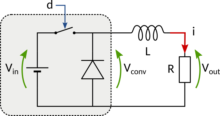
Fig. 4.1 Buck converter feeding a RL load: an example of hybrid system, that is a blend of continuous and discrete behaviors.

Objective: write the equations to simulate voltage \(V_{out}\) and current \(i\).

Modeling method: by considering that the diode is always conducting, the buck converter, as seen by the RL load, is equivalent to a voltage source which is either equal to \(V_{in}\) (when switch is closed) or 0 (when switch is open and diode is closed). Such a switching signal with a constant duty cycle can be written with the modulo on the time variable.

Syntax for the modulo function can be found in the ModelicaReference/Operators documentation, available in OMEdit libary browser (also online).

Parameters:

input voltage Vin	switching period T	resistance R	inductance L
5 V	1 ms	1 Ω	3 mH

4.2. State event: diode rectifier

We illustrate state events with the simplest diode rectifier, the half-wave rectifier which uses just one diode (Fig. 4.2). Power supply is a sinusoidal voltage source (amplitude 1 V, frequency 3 Hz). It feeds through the diode a resistive load (R=1 Ω) in parallel with a capacitive filter (C = 1 F). Simulation time should be 1 s.

Fig. 4.2 Half-wave diode rectifier feeding a RC load: an example of hybrid system, that is a blend of continuous and discrete behaviors.

Objective: write a flat textual model (i.e. not based on Modelica.Electrical components) of the circuit. We’ll do this in two steps:

1. first, the diode will simply have the behavior of a resistance Ron.

   • check that you get an reasonable capacitor voltage.

   • what happens when Ron is set to zero?

2. then, use the if keyword to set the diode current to zero when its voltage is negative. You should use a piecewise defined equation for the current.

   • check that you get the classical behavior of a diode rectifier.

   • what happens when the number of simulation point is small (ex : 10) ?

You can use the following lines to declare the variables and parameters:

import Modelica.Units.SI.{Voltage, Current, Resistance, Conductance, Capacitance, Frequency};
import Modelica.Constants.pi;

Voltage u, vd, vr, vc;
Current i, ir, ic;
parameter Resistance R=1;
parameter Capacitance C=1;
parameter Frequency f=3;