7. Custom components

In the Physical components chapter, we’ve seen how to use Modelica components, in particular components from the Modelica Standard Library. In this session, you’ll create new custom components. To do so, you’ll learn what components are made of, in particular Connector objects.

Main ressource needed: Michael Tiller’s online book “Modelica by Example” [Tiller-2014]

chapter Connectors (e.g. the intro and the review on Connector Definitions)
chapter Components

7.1. Thermistor

For this work, you need to download an save the ThermistorPackage ThermistorPackage.mo.

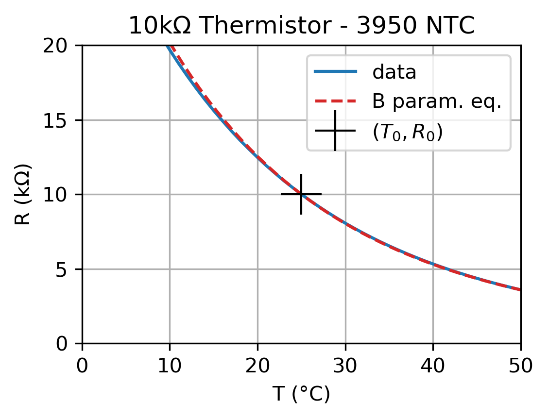
Background theory: a thermistor is a resistor whose resistance depends on temperature. In particular, NTC thermistors are typically used as temperature sensors. Their resistance decreases with temperature, with a relationship typically described with the so-called “B parameter equation”:

\[\frac{1}{T} = \frac{1}{T_0} + \frac{1}{B}\ln \left(\frac{R}{R_0}\right)\]

where \(R_0\) is the resistance at a reference temperature \(T_0\) (25°C for example) and \(B\) is the gain (slope of \(ln(R)\) vs \(1/T\)). The following plot is the \(R(T)\) relationship for a 10 kΩ thermistor “NTC 3950” with coefficient \(B\) equal to 3950, thus the name.

Objective: implement the Thermistor component using this \(R(T)\) relation.

the Thermistor component should work when connected with the provided TestBlank model. Thus it should have two electrical Pins (connector from Modelica.Electrical.Analog) and one Heatport (from Modelica.Thermal.HeatTransfer).
the parameters of the \(R(T)\) relation should be tunable.
the package provided contains the first few lines

Remark:

A good modeling practice, based on the DRY principle (see chapter Organizing models), would suggest that the Thermistor model should inherit from Modelica.Electrical.Analog.Interfaces.OnePort. However, the objective here is to understand how to build acausal components from scratch, so we give up on inheritance in this specific case.

Visual touch:

Edit in the “Icon view” the appearance of the component so that it looks like a kind of resistance.
Add text with the placeholders for some parameters (like B=%B) so that the user can have an immediate view the their value. Similarly, you can use %name to show the name of the component instance.

7.1.1. Advanced version

If you’ve finished the Thermistor, you can complexify its equation to allow the user to switch between 3 different model types:

linear model (with a first-order temperature coefficient)
B parameter equation (used above)
and the more accurate Steinhart–Hart equation.

You can use an Enumeration to hold the model kind. The if statement (cf. the If section in Modelica by Example) enables the conditional definition of the \(R(T)\) behavior equation.

7.1.2. Custom parameter tuning dialog

As a final touch, you can use the Dialog annotation to get a well-organized parameter tuning dialog (i.e. the small window popping up when double-clicking a component). This annotation is heavily used in complex components such as those in Modelica.Electrical.Machines:

final parameter Modelica.SIunits.Temperature TpmOperational=293.15
    "Operational temperature of permanent magnet"
    annotation (Dialog(group="Operational temperatures"));

7.2. Electro active damper

The 2nd supporting example of this session is to enhance the component-based vehicle suspension with what can be found in some luxury cars: an electro active damper. You will replace the existing mechanical damper by an electrical generator. Then, this generator can be connected to a resistor (which yields the same behavior as the mechanical damper), or use a more complex electronical circuitry.

The key component for such a generator is an EMF, like the one found in the model of DC motors, but within the translational mechanical domain, rather than the usual rotational EMF.

7.2.1. Organization of the work

To create such an electromechanical components, it is useful to take inspiration from existing standard electrical and mechanical components, like the Damper or the Resistor. This is made possible by the opensource nature of MSL.

As a first step, we will create a custom mechanical-only component which will behave exactly like the MSL Damper, but where we have full control over the code.

Then, we will complexify this model to add the two necessary electrical pins and implement the EMF equation.

Testing

For testing purpose, you will connect the EMF electrical port to a resistance which value will be computed so as to generate the exact same behavior as the damper with damping factor a.

7.2.2. Custom mechanical component

This Damper model from Modelica.Mechanics.Translational.Components is defined within the single-file package Translational.mo. You can open this MSL file with any text editor but, in OMEdit, the most convenient way to look at this model is two use “Open Class” action from the context menu in OMEdit.

Damper code:

model Damper "Linear 1D translational damper"
  extends Translational.Interfaces.PartialCompliantWithRelativeStates;
  parameter SI.TranslationalDampingConstant d(final min=0, start=0)
    "Damping constant";
  extends
    Modelica.Thermal.HeatTransfer.Interfaces.PartialElementaryConditionalHeatPortWithoutT;
equation
  f = d*v_rel;
  lossPower = f*v_rel;

  annotation (/*…*/);
end Damper;

This Damper model extands a base (partial) model PartialCompliantWithRelativeStates, defined within Modelica.Mechanics.Translational.Interfaces (in the same Translational.mo file):

partial model PartialCompliantWithRelativeStates
  "Base model for the compliant connection of two translational 1-dim. shaft flanges where the relative position and relative velocities are used as states"

  parameter StateSelect stateSelect=StateSelect.prefer
    "Priority to use phi_rel and w_rel as states"
    annotation (HideResult=true, Dialog(tab="Advanced"));
  parameter SI.Distance s_nominal=1e-4
    "Nominal value of s_rel (used for scaling)"
    annotation (Dialog(tab="Advanced"));

  SI.Position s_rel(
    start=0,
    stateSelect=stateSelect,
    nominal=s_nominal) "Relative distance (= flange_b.s - flange_a.s)";
  SI.Velocity v_rel(start=0, stateSelect=stateSelect)
    "Relative velocity (= der(s_rel))";

  SI.Force f "Forces between flanges (= flange_b.f)";
  Translational.Interfaces.Flange_a flange_a
    "Left flange of compliant 1-dim. translational component" annotation (
      Placement(transformation(extent={{-110,-10},{-90,10}})));
  Translational.Interfaces.Flange_b flange_b
    "Right flange of compliant 1-dim. translational component" annotation (
      Placement(transformation(extent={{90,-10},{110,10}})));

equation
  s_rel = flange_b.s - flange_a.s;
  v_rel = der(s_rel);
  flange_b.f = f;
  flange_a.f = -f;

  annotation (/*…*/);
end PartialCompliantWithRelativeStates;

With these code extracts, you should be able to create a custom ElecMechConv class, defined within your Suspension package created in the previous section. As a first step, this component should behave exactly as the Damper.

7.2.3. Custom electro-mechanical component

Resistor (defined within Modelica.Electrical.Analog.Basic package in the /usr/lib/omlibrary/Modelica 3.2.2/Electrical/Analog/Basic.mo file):

model Resistor "Ideal linear electrical resistor"
  parameter SI.Resistance R(start=1)
    "Resistance at temperature T_ref";
  parameter SI.Temperature T_ref=300.15 "Reference temperature";
  parameter SI.LinearTemperatureCoefficient alpha=0
    "Temperature coefficient of resistance (R_actual = R*(1 + alpha*(T_heatPort - T_ref))";

  extends Modelica.Electrical.Analog.Interfaces.OnePort;
  extends Modelica.Electrical.Analog.Interfaces.ConditionalHeatPort(T=T_ref);
  SI.Resistance R_actual
    "Actual resistance = R*(1 + alpha*(T_heatPort - T_ref))";

equation
  assert((1 + alpha*(T_heatPort - T_ref)) >= Modelica.Constants.eps,
    "Temperature outside scope of model!");
  R_actual = R*(1 + alpha*(T_heatPort - T_ref));
  v = R_actual*i;
  LossPower = v*i;

  annotation (/*…*/);
end Resistor;

and Resistor extends partial model OnePort (defined within Modelica.Electrical.Analog.Interfaces):

partial model OnePort
  "Component with two electrical pins p and n and current i from p to n"

  SI.Voltage v "Voltage drop between the two pins (= p.v - n.v)";
  SI.Current i "Current flowing from pin p to pin n";
  PositivePin p
    "Positive pin (potential p.v > n.v for positive voltage drop v)" annotation (Placement(
        transformation(extent={{-110,-10},{-90,10}})));
  NegativePin n "Negative pin" annotation (Placement(transformation(extent={{
            110,-10},{90,10}})));
equation
  v = p.v - n.v;
  0 = p.i + n.i;
  i = p.i;

  annotation (/*…*/);
end OnePort;

Using inspiration from these classes, you should expand your ElecMechConv component to add two electrical pins.

The equation for a translational EMF are adapted from the EMF of the usal (rotational) DC motor:

\[u = K.v, f = K.i\]

where \(K\) is the translational emf constant (in V/(m/s) or N/A), \(u,i\) are the electrical voltage and current, and \(v,f\) the mechanichal velocity and force. Notice that the name of the variables in this equation should be adapted to match the names used in the Modelica code.

7.2.4. Appearance: Icon View

Use the “Icon View” of OMEdit to customize the appearance of your ElecMechConv component. In particular:

place the four connectors at reasonable places
add an artistic touch to give a distinctive appearance of the EMF block in the general suspension model.

Also, you can use the %name text, which will be replaced by the actual name of the component.