2. Introduction to the Grid Connected Inverter

Learning objectives

In this session, you’ll learn:

1. the basic principle of AC power transmission
2. the topology of the three phase (two-level) voltage source inverter
3. how to make a time domain simulation of such a converter, using Simulink/SimPowerSystems (open loop simulation, without the power flow control)

2.1. Preamble: AC Power transmission

Before entering the details of a grid connected inverter, we need to understand the basic principle of power transmission between two AC voltage sources. To this end, let’s study the circuit represented on Fig. 2.1. Notice that this diagram is the single phase equivalent circuit of a balanced three phase circuit.

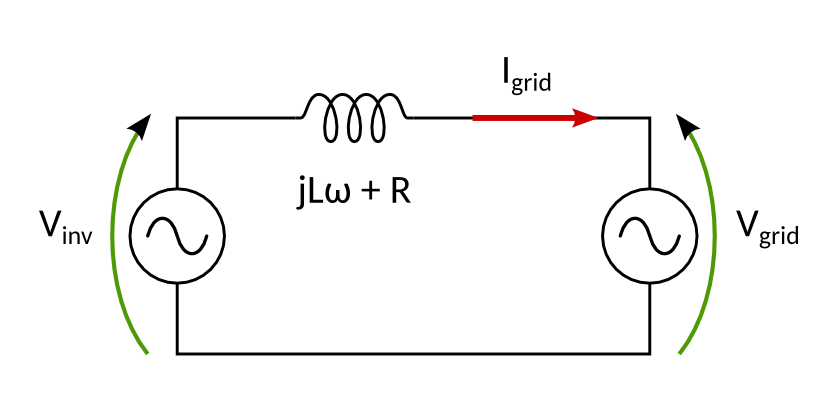
Fig. 2.1 Power transfer between two voltage sources (e.g. an inverter and the grid) through an inductive line

The power flow can be explained in sinusoidal regime using complex representations for the voltages and currents. These complex amplitudes can then be represented on a phasor diagram. When working with complex currents, it is usual to use a polar notation like \(\underline{I} = Ie^{-j\phi}\), with \(\phi\) the phase lag with respect to a reference (grid voltage for example), and \(I\) the amplitude. However, for reasons that will become clearer after, it will be better in this control lab to express complex amplitudes in cartesian coordinates: \(\underline{I} = I_d + j I_q\) [1]. The grid voltage is taken the phase reference, so \(\underline{V}_{grid} = V_g\) (a real number).

Question

Relate the active and reactive power (“P” and “Q”) received by the grid to the current components \(I_d, I_q\) and the amplitude of the grid voltage \(V_g\). You may need to remember the definition of complex power.

Now, for a given grid voltage, the current flowing between the two sources is in fact controlled by the inverter voltage \(\underline{V}_{inv} = V_d + j V_q\).

Question

Relate the current components \(I_d, I_q\) to the inverter voltage components \(V_d, V_q\). Then combine this relation with the previous one to conclude on the influence of \(V_d, V_q\) on \(P, Q\). (relationships are simpler when supposing that the resistance is negligible: \(R << L\omega\).).

You can apply the formula to fill in this table:

desired power	P=0, Q=0	P>0, Q=0	P=0, Q>0
\(V_d\)
\(V_d\)

Also, you can draw a phasor diagram, taking the fixed grid voltage as a reference, to visualize how the inverter voltage influence the current flowing through the inductor, and thus the power flows. You can use Geogebra to make an interactive geometric drawing.

Keeping these results in mind, we can now turn to the real inverter, with two changes

• three-phase system
• PWM operation

2.2. System under study

We consider a 20 kVA three phase two-level inverter, which is one of the key parts of a PV power plant. The inverter is made of three inverter legs, each made of two electronic switches (probably implemented with IGBT technology).

The topology of the inverter is given on Fig. 2.2. The DC voltage source is a simplified representation of the power generation by the PV panels.

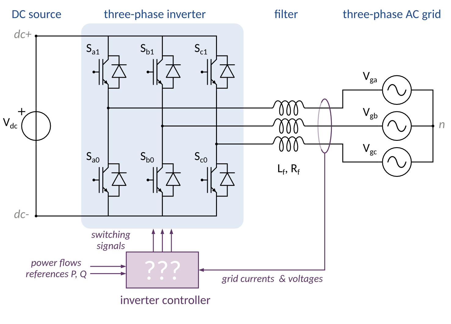
Fig. 2.2 Topology of a three-phase grid connected inverter, along with the abstract structure of the power flow control.

2.2.1. Model parameters

grid filter:

• inductance Lf = 2 mH
• series resistance Rf = 10 mΩ

Switching frequency fs = 20kHz

Voltage on the DC link: Vdc = 700 V

Grid voltage: 230/400 V

2.3. Simulink wiring

We will run numerical simulations using Simscape Power Systems (formerly SimPowerSystems) toolbox for Simulink. This toolbox enables physical modeling in Simulink, i.e. based on acausal models, as opposed to block diagram which are causal models.

Do not hesitate to look at Simscape Power Systems documentation, in particular the guide on how to Build and Simulate a Simple Circuit. Before wiring the full inverter, you can start with the simpler schematic of Fig. 2.1.

Question (main objective of this session)

Make an open loop simulation of the three phase inverter, in a way where you can easily change the d and q components of the inverter voltage.

2.3.1. Some useful blocks

Powergui

To simulate any SimPowerSystems model, a powergui block is needed. As explained in the Build and Simulate a Simple Circuit tutorial, it is used to store the equivalent Simulink circuit that represents the state-space equations of the SimPowerSystems blocks.

PWM generator

To generate the 6 switching signals out of the duty cycle signals (3 duty cycles, one for each leg), a PWM genetor (also sometimes called modulator) is needed.

SimPowerSystems provides a PWM Generator (2-Level) block for this purpose. Its output is a vector of 6 switching signals, so that a demux block is needed (cf. Fig. 2.3).

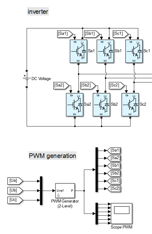
Fig. 2.3 Wiring of the PWM Generator for the three phase inverter. Notice the ordering of the switching signals.

In principle, one could expect that the inputs are unitless (duty cycles between 0 and 1). However, the min-max option of this block can be chosen so that the input has a more convenient range.

Question

How to set the min-max option of the PWM generator so that the three input signals corresponds to the phase-to-ground voltage of each leg ?

Notice that there are many ways to generate PWM signals, using different modulation techniques (e.g. Space Vector Modulation). We won’t cover the modulation in this lab.

Measurements

Current and Voltage measurement blocks are needed to extract signals from the SimPowerSystems simulation. Then these signals can then be sent to regular a Simulink scope for example.

2.4. PMW: moving average value

When looking at the output voltages of the inverter, you’ll notice how difficult it is to visualize the underlying average value.

Question

How to visualize the average of PWM voltages ?

Footnotes

[1]	“d” and “q” stand for “direct” and “quadrature” axes respectively. They will be detailed when introducing the dq (Park) transform (TODO: ref).