2. Grid simulation
Objective of the session:
- derive the equations of the network
- solve these equations numerically using a backward-forward algorithm
2.1. Modeling
2.1.1. Network description
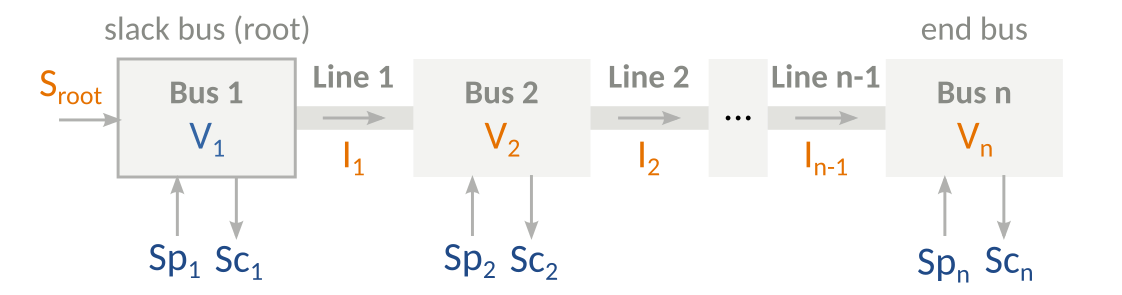
Fig. 2.1 Topology of the distribution network (linear structure). Fixed quantities (input data) in blue, unknown quantities in orange.
Root (busbar) voltage: 20.4 kV line-to-line, 0° (1.02 pu).
As a starting point, we consider the simplest test case possible, with \(n_b=3\) buses (and thus \(n_l=2\) lines). Notice that for a radial network, the relation \(n_b=n_l+1\) always holds (property of a tree graph).
test case data:
| Bus | Production | Consumption |
|---|---|---|
| 1 | 0 | 0 |
| 2 | 3 MW + 0 MVAR | 4 MW + 1.6 MVAR |
| 3 | 3 MW + 0 MVAR | 4 MW + 1.6 MVAR |
2.1.2. Line model
A “Pi model” is used for lines:
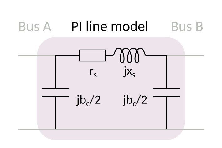
Fig. 2.2 Pi model for a line (branch) of the network
| Parameter | Value | Unit |
|---|---|---|
| series resistance rs | 0.5 | Ω/km |
| series reactance xs | 0.25 | Ω/km |
| charging susceptance [1] bc | 3.5e-5 | S/km |
These are linear quantities (values per unit of length), that need to be multiplied by the length of each line. For are test case with 2 lines:
| Line 1 (bus 1 - bus 2) | 12 km |
| Line 2 (bus 2 - bus 3) | 15 km |
2.1.3. Per-unit system
The per-unit system is widely used notation to replace SI units (V,A,W) by dimensionless quantities.
For example, an actual voltage \(V_{SI}\) (in Volts) is replaced by a per unit value \(V_{pu}\) by dividing it with a base voltage \(V_0\):
A base quantity is needed for each unit we want to normalize: voltage, current, resistance,… However, to preserve physical equations (S=VI, V=ZI), these base quantities are derived from each others. In the end, only 2 base quantities need to be chosen:
- Base voltage \(V_0\): chosen as the rated voltage of the network [2].
- Base power \(S_0\): chosen as a round value, whose order of magnitude should relate to the ratings of the system.
For the medium voltage grid considered in this lab, we choose then
| \(V_0\) | 20 kV (phase to phase) |
| \(S_0\) | 1 MVA |
Example: a 20.4 kV voltage is represented by a 20.4/20 = 1.02 pu voltage
Derived base quantities
From these two base values only, we can derive the other base quantities.
For example, because of the relation \(\underline{S} = P+jQ\), the base quantities for active and reactive power should be chosen the same as \(S_0\).
Current: to preserve the equation for complex power (\(\underline{S} = \underline{V}\underline{I}^*\)), the base current need to be chosen as:
Impedance: to preserve Ohms’s law (\(\underline{V} = \underline{Z}\underline{I}\)), he base current need to be chosen as:
This base impedance applies also to normalize resistances and reactances. Its inverse, the base admittance (\(Y_0 = 1/Z_0\)) applies also to normalize conductances and susceptances.
Three phase system
The equations for base current and base impedance depends on the power equation and Ohm’s law, which are different in 3 phase systems.
In the case where we work with line-to-line voltages, we have \(\underline{S} = \sqrt{3}\underline{V}\underline{I}^*\), so base current should be:
and similarly, because \(\underline{V} = \sqrt{3}\underline{Z}\underline{I}\), the base impedance should be:
Then, when quantities are normalized using these base values, the \(\sqrt{3}\) factor disappears from the power equation and Ohm’s law: equations are the same as for a single phase system!
Question
In your Matlab script, define variables for the base quantities: start with 20 kV and 1 MVA, and then implement the above relations for the derived quantities.
2.2. Power flow
A power flow algorithm aims at computing the unknown voltages and currents in a network. There are many good quality implementation available (both commercial and free), which leverage on decades of R&D on this topic. This means in practice it is not a good idea to rewrite your own solver.
However, for the special case a radial network, there exists an algorithm called “backward-forward method” [Shi88]. It is both efficient (convergence in about 10 iterations) and much easier to implement than general purpose power flow method (like those based on Newton-Raphson method).
2.2.1. Description of the backward-forward method
The method is iterative, starting with an initial guess of bus voltages.
Each iteration involves two successive steps:
- a backward sweep to compute the line currents, using the curent law (KCL). It starts from the end node, and goes upstream iteratively. At each next bus, the downstream current is summed with all currents injected at the bus to compute the upstream current.
- a forward sweep, to update the estimates of the bus voltages, using the voltage law (KVL). It starts from the root node (busbar) where the voltage is known, and goes downstream iteratively to the end node by substracting the voltage drop on the downstream line (using Ohm’s law and previously computed line currents).
Be careful that during the backward phase (current computation), the bus voltages are not updated. Similarly, line currents are not updated during the forward phase.
These two steps are repeated until a convergence criterion is met, or a maximum number of iterations is met (no more than 20 should be needed, otherwise something is broken).
Question
Implement the backward-forward algorithm to solve the power flow in the test network above.
Should be working with any number of nodes.
Numerical results to self check the correctness of your code:
bus 1: voltage 1.0200 pu, 0.00°
bus 2: voltage 0.9642 pu, 1.69°
bus 3: voltage 0.9286 pu, 2.90°
line currents: 108.4, 56.3 A
S_root =  2.2828 + 2.9877i pu
2.3. Refactoring
Once the algorithm is working, it should be packaged in a function with a well defined API, for further reuse. In particular, choose:
- a nice set of input parameters
- a nice set of output values
avoid global variables unless they really make sense…
2.3.1. Stress test of the power flow
A test case to check the flexibility of your power flow routine AND answer an interesting question: instead of using one Pi model for each line, use a series of smaller Pi segments (with rescaling of impedances), for example one segment per kilometer. Power injections should be kept at the same distances of the root bus.
Then, make a nice plot to compare the voltage profile (magnitude and angle) and current along the length of the grid. Is there is big difference?
Footnotes
| [1] | A susceptance B is the imaginary part of an admittance Y = G+jB, in siemens. G is a conductance, but it is generally approximated to 0 for a grid line. |
| [2] | If the network include transformers, meaning that parts of the system operate at different voltage, then a different base voltage is chosen for each subsystem. Doing so yields the nice property that ideal transformers disappear from per-unit equations: a transformer is then only represented by its leakage impedance. |
2.4. Power flow with Matpower
http://www.pserc.cornell.edu/matpower/
Creating the “Matpower test case” (mpc).
Python script to generate the Matlab structure from an Excel spreadsheet:
excel_matpower_converter.zip.
Question
Create the Matpower test case for the 3 bus grid described above.